Moment Analysis Tutorial

Theory

This tutorial will follow the work of Boris Grube (see this repository for a much more in-depth set of scripts). I will shortly summarize his work and show how it can be applied via laddu.

First, let’s define what a moment is. In physics, the first first time we hear about moments is probably in discussions of moments of inertia, which is calculated as

\[\int \int \int \rho(\vec{r}) ||\vec{r}||^2 \text{d}V\]

where \(\rho\) is the mass density function. We see similar definitions for statistical moments like the mean, variance, and so on, where the general idea involves integrating over some function which defines a phase space of the data times some other function which we want to interrogate. In the moment of inertia, we are adding up all of the contributions from every point in an object, where the contribution is weighted by its distance from some point (typically the point of rotation).

On the other hand, in particle physics, a moment analysis is an integral over the phase space of decay angles, and the quantity we wish to extract is a simple complex coefficient. While these concepts are similar, the particle physics moment is more closely related to a generalized Fourier expansion. Rather than sine and cosine waves, we will expand the angular distribution of decay products into a basis of spherical harmonics.

Since the spherical harmonics form a complete orthonormal basis, we can expand any angular distribution as follows:

\[I(\theta, \varphi) = \sum_{LM}^{\infty} H(L,M) Y_L^M(\theta, \varphi)\]

We can then calculate moments as

\[H(L, M) = \int_{4\pi} \text{d}\Omega I(\Omega) Y_L^{M*}(\Omega)\]

where \(\Omega\) is shorthand for the solid angle, such that \(\int_{4\pi}\text{d}\Omega = \int_{-1}^{+1}\text{d}\cos\theta \int_{-\pi}^{\pi}\text{d}\varphi\). We typically normalize spherical harmonics with a factor of \(N_L = \sqrt{\frac{2 L + 1}{4\pi}}\), so we will actually write

\[H(L, M) = \frac{1}{N_L} \int_{4\pi} \text{d}\Omega I(\Omega) Y_L^{M*}(\Omega)\]

However, technically the intensity must be purely real, so with a bit of math we actually write

\[I^{\text{meas}}(\theta, \varphi) = \sum_{LM}^{\infty} (2 - \delta_{M0}) \Re[H(L,M) Y_L^M(\theta, \varphi)]\]

where the delta-function arises from the fact that the \(M=0\) spherical harmonics are already purely real. In practice, we calculate moments as

\[H(L, M) = \frac{1}{N_L} \int_{4\pi} \text{d}\Omega (2 - \delta_{M0}) I^{\text{meas}}(\Omega) Y_L^{M*}(\Omega)\]

which, for discrete data, becomes

\[H(L, M) \approx \frac{1}{N_L} \sum_{i}^{\text{data}} (2 - \delta_{M0}) Y_L^{M*}(\Omega_i)\]

and we only consider the real part of \(H(L, M)\).

Implementation

To implement this in code, we could imagine a function like

import laddu as ld
import numpy as np

def get_moment(data: ld.Dataset, *, l: int, m: int) -> complex:
    n_l = np.sqrt((2 * l + 1) / (4 * np.pi))
    beam = ld.Particle.stored('beam')
    target = ld.Particle.missing('target')
    kshort1 = ld.Particle.stored('kshort1')
    kshort2 = ld.Particle.stored('kshort2')
    kk = ld.Particle.composite('kk', [kshort1, kshort2])
    proton = ld.Particle.stored('proton')
    reaction = ld.Reaction.two_to_two(beam, target, kk, proton)
    angles = reaction.decay('kk').angles('kshort1')
    ylm = ld.Ylm('ylm', l=l, m=m, angles=angles)
    model = ylm.conj() # take the conjugate
    evaluator = model.load(data)
    values = evaluator.evaluate([]) # no free parameters
    weights = data.weights # we can also include weighted events here
    return np.sum(weights * values) / n_l * (2 if m != 0 else 1)

In principle, we can run this method for any \(L \geq 0\) and \(-L \leq M \leq L\), but note the symmetry property of the spherical harmonics:

\[Y_L^{M*}(\Omega) = (-1)^M Y_L^{-M}(\Omega)\]

which means we really only need to calculate \(0 \leq M \leq L\). The code to do this is also fairly simple:

l_max = 4 # we need to truncate at some maximum value, we can't use infinity!
moments = np.array([get_moment(data, l=l, m=m) for l in range(l_max + 1) for m in range(l + 1)])

We could go ahead and plot these, but there is one further consideration before we do, and that is the efficiency of the detector. In an extended maximum likelihood fit, we use accepted phase-space Monte Carlo events to approximate a normalization integral, the integral of the acceptance function \(\eta(\Omega)\) over the entire angular phase space. We do this with Monte Carlo because in practice, we don’t have an analytical form for the acceptance function and can only understand it by passing many phase-space distributed events through a simulation of the detector.

Theory (again)

When we include acceptance, we find that the spherical harmonics take the form

\[\begin{split}H^{\text{meas}}(L, M) &= \frac{1}{N_L} \int_{4\pi} \text{d}\Omega I^{\text{meas}}(\Omega) Y_L^{M*}(\Omega) \\ &= \frac{1}{N_L} \int_{4\pi} \text{d}\Omega I(\Omega) \eta(\Omega) Y_L^{M*}(\Omega)\end{split}\]

Using the definition for \(I(\Omega)\) (which uses the real part of the spherical harmonics), we find

\[H^{\text{meas}}(L, M) = \sum_{L'M'} H(L', M') \frac{N_{L'}}{N_L} (2 - \delta_{M'0}) \int_{4\pi} \text{d}\Omega \Re[Y_{L'}^{M'}(\Omega)] \eta(\Omega) Y_L^{M*}(\Omega)\]

We can then define a matrix of acceptance integrals,

\[I^{\text{acc}}_{LML'M'} = \frac{N_{L'}}{N_L} (2 - \delta_{M'0}) \int_{4\pi} \text{d}\Omega \Re[Y_{L'}^{M'}(\Omega)] \eta(\Omega) Y_L^{M*}(\Omega)\]

such that

\[\vec{H}^{\text{meas}} = I^{\text{acc}} \vec{H}\]

where the notation \(\vec{H}\) corresponds to an arbitrarily ordered vector of all moments \(H(L, M)\) (arbitrary as long as we keep the ordering consistent throughout the calculation). We then invert the acceptance matrix to transform the measured moments into the true, physical moments.

To calculate this matrix, we again convert the integral over the acceptance function to a sum over accepted Monte Carlo, normalized by the size of the generated dataset. We could possibly be a bit more precise and find some way to calculate the normalization from some evaluation of moments over the generated data, but for this tutorial we’ll just use the total number of events:

\[I^{\text{acc}}_{LML'M'} \approx \frac{N_{L'}}{N_L} (2 - \delta_{M'0}) \frac{4\pi}{N_{\text{gen}}} \sum_{i}^{\text{accmc}} \Re[Y_{L'}^{M'}(\Omega_i)] Y_L^{M*}(\Omega_i)\]

Note the additional factor of \(4\pi\) here, which is another normalization choice.

Implementation

Again, we can write this in code in a rather simple way:

def get_norm_int_term(
    accmc: ld.dataset,
    *,
    n_gen: int,
    l: int,
    m: int,
    l_prime: int,
    m_prime: int,
) -> complex:
    n_l = np.sqrt((2 * l + 1) / (4 * np.pi))
    n_l_prime = np.sqrt((2 * l_prime + 1) / (4 * np.pi))
    beam = ld.Particle.stored('beam')
    target = ld.Particle.missing('target')
    kshort1 = ld.Particle.stored('kshort1')
    kshort2 = ld.Particle.stored('kshort2')
    kk = ld.Particle.composite('kk', [kshort1, kshort2])
    proton = ld.Particle.stored('proton')
    reaction = ld.Reaction.two_to_two(beam, target, kk, proton)
    angles = reaction.decay('kk').angles('kshort1')
    ylm = ld.Ylm('ylm', l=l, m=m, angles=angles)
    ylm_prime = ld.Ylm('ylm_prime', l=l_prime, m=m_prime, angles=angles)
    model = ylm.conj() * ylm_prime.real()
    evaluator = model.load(accmc)
    values = evaluator.evaluate([]) # no free parameters
    weights = accmc.weights # only needed if the accepted MC is weighted
    return np.sum(weights * values) * n_l_prime / n_l * (2 if m_prime != 0 else 1) * 4 * np.pi / n_gen

l_max = 4
measured_moments = np.array([get_moment(data, l=l, m=m) for l in range(l_max + 1) for m in range(l + 1)])
norm_int = np.array([
    [
        get_norm_int_term(accmc, n_gen=n_gen, l=l, m=m, l_prime=l_prime, m_prime=m_prime)
        for l_prime in range(l_max + 1) for m_prime in range(l_prime + 1)
    ]
    for l in range(l_max + 1) for m in range(l + 1)
])
norm_int_inv = np.linalg.inv(norm_int)
physical_moments = np.dot(norm_int_inv, measured_moments)

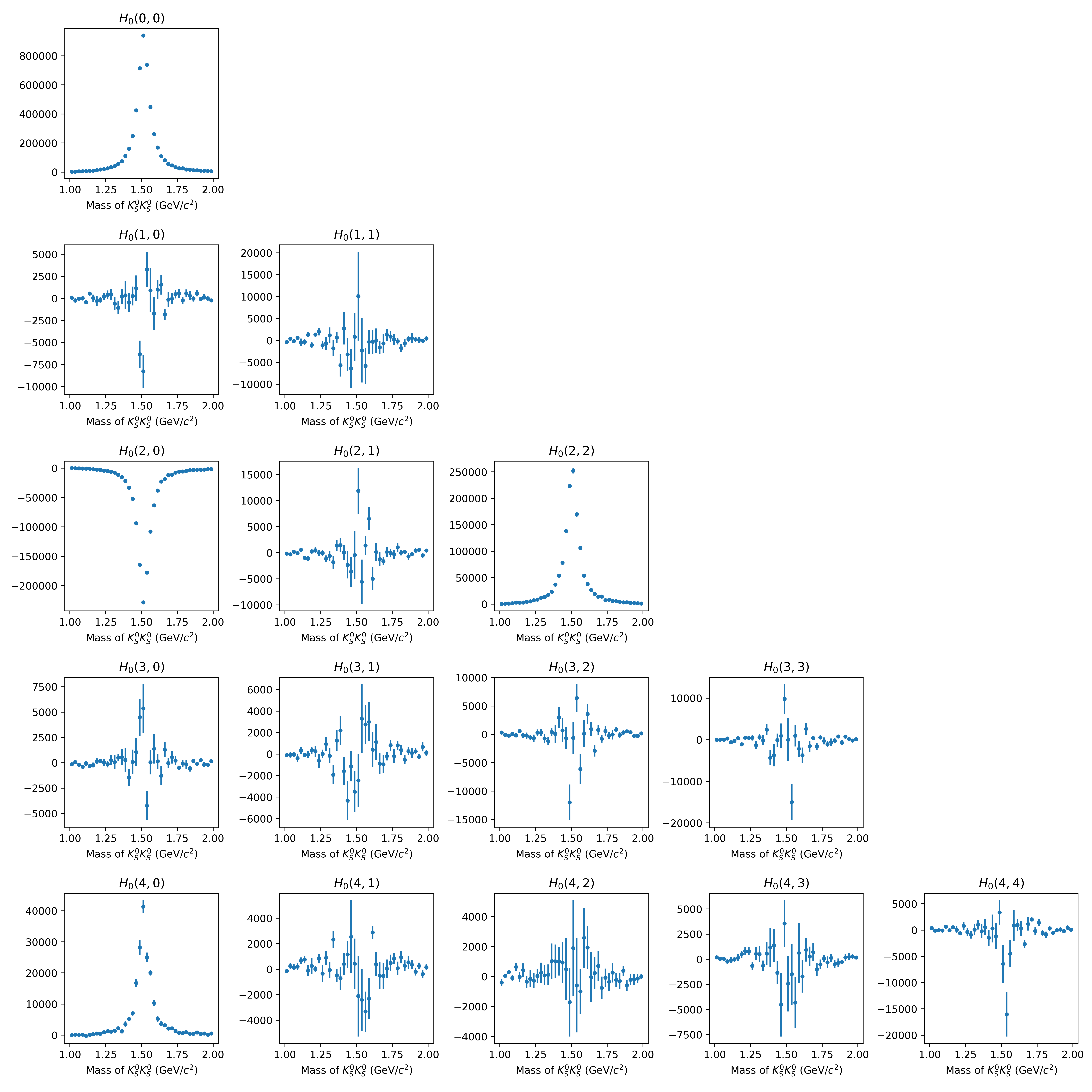
Once we have the physical moments, we can plot them or use them to perform other analyses. Some theory models predict certain distributions of moments with respect to Mandelstam variables or invariant masses, for example. We can plot the distribution here in bins of invariant mass, binning our data in a similar way to the Binned Fitting Tutorial. I’ll leave the code as an exercise, but if you get stuck, example_2 in the laddu repository is a complete working program which will also do the additional step of calculating polarized moments assuming a linearly polarized photon beam experiment. That example also goes through the process of bootstrapping the moments to estimate their uncertainty, although there are also methods to propagate the uncertainty from the measured covariance matrix. The result of such an analysis might look something like this (note that these are what we call “unnormalized moments”, where normalized moments would be normalized such that \(H(0,0) = N_{\text{data}}\)):