Unbinned Fitting Tutorial

Theory

Perhaps the simplest kind of fitting we can do with laddu is one which involves fitting all of the data simultaneously to one model. Suppose we have some data representing events from a particular reaction. These data might contain resonances from intermediate particles which can be reconstructed from the four-momenta we’ve recorded, and those resonances have their own observable properties like angular momentum and parity. We can construct a model of these resonances in both mass \(m\) and angular space \(\Omega\) and define \(p(x; m, \Omega)\) to be the probability that an event \(x\) has the given phase space distribution. Since we also observe events themselves in a probabilistic manner, we must also consider the probability of observing \(N\) events from such a process. This can be done with an extended maximum likelihood, following the derivation by [Barlow]. First, we admit that while we defined \(p(x; m, \Omega)\), we assumed it would have unit normalization. However, we will now consider replacing this with a function whose normalization is not so constrained, called the intensity:

\[\int \mathcal{I}(x; m, \Omega) \text{d}x = \mathcal{N}(m, \Omega)\]

We do this because our observed number of events \(N\) will deviate from the expected number predicted by our model (\(\mathcal{N}(m, \Omega)\)) according to Poisson statistics, since the observation of events themselves is a random process and are also subject to the efficiency of the detector (which we will discuss later).

Of course, we now have the problem of maximizing the resultant likelihood from this unnormalized distribution. We can write the likelihood using a Poisson probability distribution multiplied by the original product of probabilities over each observed event:

\[\begin{split}\mathcal{L} &= e^{-\mathcal{N}}\frac{\mathcal{N}^N}{N!} \prod_{i=1}^{N} p(x_i; m, \Omega) \\ &= \frac{e^{-\mathcal{N}}}{N!} \prod_{i=1}^{N} \mathcal{I}(x_i; m, \Omega)\end{split}\]

given that the extended probability is related to the standard one by \(\mathcal{I} = \mathcal{N} p\). Next, we will consider that the efficiency of the detector can be modeled with a function \(\eta(x)\). In reality, we generally cannot know this function to any level where it would be useful in such a minimization, but we can approximate it through a finite sum of simulated events passed through a simulation of the detector used in the experiment. We will then say that

\[\mathcal{N}'(m,\Omega) = \int \mathcal{I}(x; m, \Omega)\eta(m, \Omega)\text{d}x\]

gives the predicted number of events with efficiency encorporated, so

\[\mathcal{L} = \frac{e^{-\mathcal{N}'}}{N!}\prod_{i=1}^{N}\mathcal{I}(x_i; m, \Omega)\eta(m, \Omega)\]

While we mathematically could maximize the likelihood given above, a large product of terms between zero and one (or floating point values in general) is computationally unstable. Instead, we rephrase the problem from maximimizing the likelihood to maximizing the natural log of the likelihood, since the logarithm is monotonic and the log of a product is just the sum of the logs of the terms. Futhermore, since most optimization algorithms prefer to minimize functions rather than maximize them, we can just flip the sign. The the negative log of the extended likelihood (times two for error estimation purposes) is given by

\[\begin{split}-2\ln\mathcal{L}(x) &= -2\left(\ln\left[\prod_{i=1}^{N}\mathcal{I}(x; m, \Omega)\eta(m, \Omega)\right] - \mathcal{N}' + \ln N! \right) \\ &= -2\left(\ln\left[\prod_{i=1}^{N}\mathcal{I}(x; m, \Omega)\eta(m, \Omega)\right] - \left[\int \mathcal{I}(x; m, \Omega)\eta(m, \Omega)\text{d}x \right] + \ln N! \right) \\ &= -2\left(\left[\sum_{i=1}^{N}\ln \mathcal{I}(x; m, \Omega)\right] - \left[\int \mathcal{I}(x; m, \Omega)\eta(x)\text{d}x \right] + \ln N! + \sum_{i=1}^{N}\ln\eta(m, \Omega)\right) &= -2\left(\left[\sum_{i=1}^{N}\ln \mathcal{I}(x; m, \Omega)\right] - \left[\int \mathcal{I}(x; m, \Omega)\eta(x)\text{d}x \right]\right)\end{split}\]

The last two terms were ignored because they do not depend on the free parameters of the model, so they will only shift the likelihood surface up and down. As mentioned, we don’t actually know the analytical form of \(\eta(m, \Omega)\), but we can approximate it using Monte Carlo data. Assume we generate some data without any explicit physics model other than the phase space of the channel and pass it through a simulation of the detector. We will call these the “generated” and “accepted” datasets. We can approximate this integral a finite sum over this simulated data:

\[\int \mathcal{I}(x; m, \Omega)\eta(m, \Omega)\text{d}x \approx \frac{1}{\mathbb{P} N_g} \sum_{i=1}^{N_a} \mathcal{I}(x_i; m, \Omega)\]

where \(N_g\) and \(N_a\) are the size of the generated and accepted datasets respectively, the sum is over accepted events only, and \(\mathbb{P}\) is the area of the integration region. This last term is another unknown, but in practice, we can consider that \(\mathcal{I}\) could be rescaled by this factor, and that the multiplicative factor in the first part of the negative-log-likelihood would be extracted as the additive term \(N\ln\mathbb{P}\) which is a constant in parameter space and therefore doesn’t effect the overall minimization.

Removing all such constants, we obtain the following form for the negative log-likelihood:

\[-2\ln\mathcal{L} = -2\left(\left[\sum_{i=1}^{N}\ln \mathcal{I}(x; m, \Omega)\right] - \left[ \frac{1}{N_a} \sum_{i=1}^{N_a} \mathcal{I}(x_i; m, \Omega) \right]\right)\]

Next, consider that events in both the data and in the Monte Carlo might have weights associated with them. We can easily adjust the negative log-likelihood to account for weighted events:

\[-2\ln\mathcal{L} = -2\left(\left[\sum_{i=1}^{N} w_i \ln \mathcal{I}(x; m, \Omega)\right] - \left[ \frac{1}{N_a} \sum_{i=1}^{N_a} w_i \mathcal{I}(x_i; m, \Omega) \right]\right)\]

To visualize the result after minimization, we can weight each accepted Monte Carlo event by \(w \mathcal{L}(\text{event}) / N_a\) to see the result without acceptance correction, or we can weight each generated Monte Carlo event by \(\mathcal{L}(\text{event}) / N_a\) (generally the generated Monte Carlo is not weighted) to obtain the result corrected for the efficiency of the detector. While using \(N_a\) in the denominator is nice when you don’t have the generated Monte Carlo handy, it should generally be replaced with \(N_g\) when possible.

Example

laddu takes care of most of the math above and requires the user to provide data and the intensity function \(I(\text{event};\text{parameters})\). For the rest of this tutorial, this function will be refered to as the “model”. In laddu, we construct the model out of modular “amplitudes” (\(A(e; \vec{p})\)) which can be added and multiplied together. Additionally, since these amplitudes are functions on the space \(\mathbb{R}^n \to \mathbb{C}\), we can also take their real part, imaginary part, or the square of their norm (\(AA^*\)). Generally, when building a model, we compartmentalize amplitude terms into coherent summations, where coherent just means we take the norm-squared of the sum. Since the likelihood should be strictly real, the real part of the model’s evaluation is taken to calculate the intensity, so imaginary terms (which should be zero in practice) are discarded.

For a simple unbinned fit, we must first obtain some data. laddu does not currently have a built-in event generator, so it is recommended that users utilize other methods of generating Monte Carlo data. For the sake of this tutorial, we will assume that these data files are readily available as Parquet files.

Note

laddu only requires the column naming convention described by laddu.data.Dataset. Parquet remains the recommended container (and works in both Rust and Python), but the reader can also ingest generic ROOT TTrees via laddu.io.read_root() (either with the native oxyroot backend or backend='uproot') and, in Python, AmpTools-style ROOT tuples through laddu.io.read_amptools(). This avoids the need for any intermediate conversion scripts when working with those formats.

Reading data with laddu is as simple as using the laddu.io.read_parquet function. It takes the path to the data file as its argument:

import laddu as ld

p4_columns = ['beam', 'proton', 'kshort1', 'kshort2']
aux_columns = ['pol_magnitude', 'pol_angle']
data_ds = ld.io.read_parquet("data.parquet", p4s=p4_columns, aux=aux_columns)
accmc_ds = ld.io.read_parquet("accmc.parquet", p4s=p4_columns, aux=aux_columns)
genmc_ds = ld.io.read_parquet("genmc.parquet", p4s=p4_columns, aux=aux_columns)

Next, we need to construct a model. Let’s assume that the dataset contains events from the channel \(\gamma p \to K_S^0 K_S^0 p'\) and that the measured particles in the data files are \([\gamma, p', K_{S,1}^0, K_{S,2}^0]\). This setup mimics the GlueX experiment at Jefferson Lab (the momentum of the initial proton target is not measured and can be reasonably assumed to be close to zero in magnitude). Furthermore, because GlueX uses a polarized beam, we will assume the polarization fraction and angle are stored in the data files.

Note

The four-momenta in the datasets need to be in the center-of-momentum frame, which is the only frame that can be considered invariant between different experiments. Some of the amplitudes used will boost particles from the center-of-momentum frame to some new frame, and this is a distinct transformation from boosting directly from a lab frame to the same target frame!

Let’s further assume that there are only two resonances present in our data, an \(f_0(1500)\) and a \(f_2'(1525)\) [1]. We will assume that the data were generated via two relativistic Breit-Wigner distributions with masses at \(1506\text{ MeV}/c^2\) and \(1517\text{ MeV}/c^2\) respectively and widths of \(112\text{ MeV}/c^2\) and \(86\text{ MeV}/c^2\) respectively (these values come from the PDG). These resonances also have spin, so we can look at their decay angles as well as the overall mass distribution. Additionally, they have either positive or negative reflectivity, which is related to the parity of the exchanged particle and can be measured in polarized production (we will assume both particles are generated with positive reflectivity). These variables are all defined by laddu as helper classes:

# the mass of the combination of particles 2 and 3, the kaons
res_mass = ld.Mass(['kshort1', 'kshort2'])

# the decay angles in the helicity frame
beam = ld.Particle.stored('beam')
target = ld.Particle.missing('target')
kshort1 = ld.Particle.stored('kshort1')
kshort2 = ld.Particle.stored('kshort2')
kk = ld.Particle.composite('kk', [kshort1, kshort2])
proton = ld.Particle.stored('proton')
reaction = ld.Reaction.two_to_two(beam, target, kk, proton)
decay = reaction.decay('kk')
angles = decay.angles('kshort1')

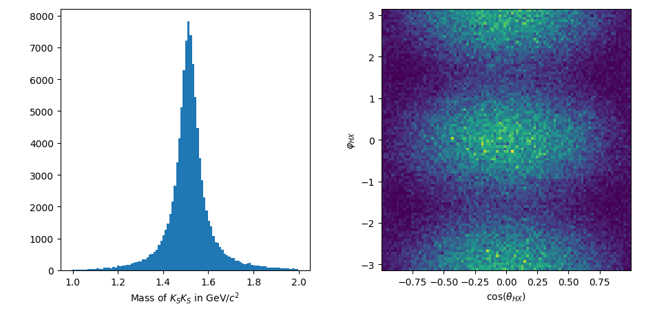
So far, these angles just represent particles in a generic dataset by index and provide an appropriate method to calculate the corresponding observable. Before we fit anything, we might want to just see what the dataset looks like:

import matplotlib.pyplot as plt

m_data = res_mass.value_on(data_ds)
costheta_data = angles.costheta.value_on(data_ds)
phi_data = angles.phi.value_on(data_ds)

fig, ax = plt.subplots(ncols=2)
ax[0].hist(m_data, bins=100)
ax[0].set_xlabel('Mass of $K_SK_S$ in GeV/$c^2$')
ax[1].hist2d(costheta_data, phi_data, bins=(100, 100))
ax[1].set_xlabel(r'$\cos(\theta_{HX})$')
ax[1].set_ylabel(r'$\varphi_{HX}$')
plt.tight_layout()
plt.show()

Next, let’s come up with a model. laddu models are formed by combining individual amplitudes using arithmetic operations as well as a few special functions for working with complex values. These terms internally keep track of all of the free parameters and caching done when a dataset is pre-computed. laddu has the amplitudes that we need already built in. We will use a relativistic Breit-Wigner to describe the mass-dependency and a \(Z_{L}^{M}\) amplitude described by [Mathieu] to fit the angular distributions with beam polarization in mind. The angular part of this model requires two coherent sums for each reflectivity, and assuming just positive reflectivity, we can write the entire model as follows:

\[\begin{split}I(m, \theta, \varphi, P_{\gamma}, \Phi) \propto &\left| [f_0(1500)] BW_0(m; m_{f_0}, \Gamma_{f_0}) \Re\left[Z_{0}^{0(+)}(\theta, \varphi, P_\gamma, \Phi)\right]\right.\\ &\left. + [f_2'(1525)] BW_2(m; m_{f_2'}, \Gamma_{f_2'}) \Re\left[Z_{2}^{2(+)}(\theta, \varphi, P_\gamma, \Phi)\right]\right|^2 \\ + &\left| [f_0(1500)] BW_0(m; m_{f_0}, \Gamma_{f_0}) \Im\left[Z_{0}^{0(+)}(\theta, \varphi, P_\gamma, \Phi)\right]\right.\\ &\left. + [f_2'(1525)] BW_2(m; m_{f_2'}, \Gamma_{f_2'}) \Im\left[Z_{2}^{2(+)}(\theta, \varphi, P_\gamma, \Phi)\right]\right|^2\end{split}\]

where \(BW_{L}(m, m_\alpha, \Gamma_\alpha)\) is the Breit-Wigner amplitude for a spin-\(L\) particle with mass \(m_\alpha\) and width \(\Gamma_\alpha\) and \(Z_{L}^{M}(\theta, \varphi, P_\gamma, \Phi)\) describes the angular distribution of a spin-\(L\) particle with decay angles \(\theta\) and \(\varphi\), photoproduction polarization fraction \(P_\gamma\) and angle \(\Phi\), and angular moment \(M\). The terms with particle names in square brackets represent the production coefficients. While these are technically both allowed to be complex values, in practice we set one to be real in each sum since the norm-squared of a complex value is invariant up to a total phase. The exact form of these amplitudes is not important for this tutorial. Instead, we will demonstrate how they can be created and combined with simple operations. First, we create a Polarization object which grabs polarization information from the dataset using the names of the beam, recoil proton, and auxiliary polarization columns:

polarization = reaction.polarization(pol_magnitude='pol_magnitude', pol_angle='pol_angle')

Next, we can create Zlm amplitudes:

z00p = ld.Zlm("Z00+", l=0, m=0, r="+", angles=angles, polarization=polarization)
z22p = ld.Zlm("Z22+", l=2, m=2, r="+", angles=angles, polarization=polarization)

The z00p and z22p objects can be combined with other amplitudes using basic math operations. The first artgument to Zlm is the name by which we will refer to the amplitude when we project the fit results onto the Monte Carlo later. Since there are no free parameters in the Zlm amplitudes, if we just built a model with these amplitudes alone, we wouldn’t have anything to minimize. Let’s now construct some amplitudes which have free parameters, particularly our production coefficients. These are the simplest amplitudes, just scalar values which are either purely real or complex. We can use the parameter function to create a named parameter in our model:

f0_1500 = ld.Scalar("[f_0(1500)]", value=ld.parameter("Re[f_0(1500)]"))
f2_1525 = ld.ComplexScalar("[f_2'(1525)]", re=ld.parameter("Re[f_2'(1525)]"), im=ld.parameter("Im[f_2'(1525)]"))

Finally, we can register the Breit-Wigners. These have two free parameters, the mass and width of the resonance. For the sake of demonstration, let’s fix the mass by passing in a parameter with a fixed value and let the width float with a parameter. These two functions create the same object, so we could just as easily write this with both values fixed or free in the fit:

bw0 = ld.BreitWigner("BW_0", mass=ld.parameter(1.506), width=ld.parameter("f_0 width"), l=0, daughter_1_mass=ld.Mass(['kshort1']), daughter_2_mass=ld.Mass(['kshort2']), resonance_mass=res_mass)
bw2 = ld.BreitWigner("BW_2", mass=ld.parameter(1.517), width=ld.parameter("f_2 width"), l=0, daughter_1_mass=ld.Mass(['kshort1']), daughter_2_mass=ld.Mass(['kshort2']), resonance_mass=res_mass)

As you can see, these amplitudes also take additional parameters like the masses of each decay product.

Next, we combine these together according to our model. For these amplitudes, we can use the + and * operators as well as real() and imag() to take the real or imaginary part of the amplitude and norm_sqr() to take the square of the magnitude (for the coherent sums). These operations can also be applied to the operated versions of the amplitudes, so we can form the entire expression given above:

positive_real_sum = (f0_1500 * bw0 * z00p.real() + f2_1525 * bw2 * z22p.real()).norm_sqr()
positive_imag_sum = (f0_1500 * bw0 * z00p.imag() + f2_1525 * bw2 * z22p.imag()).norm_sqr()
model = positive_real_sum + positive_imag_sum

Now that we have the model, we want to fit the free parameters, which in this case are the complex photocouplings and the widths of each Breit-Wigner. We can do this by creating an NLL object which uses the data and accepted Monte-Carlo datasets to calculate the negative log-likelihood described earlier.

nll = ld.NLL(model, data_ds, accmc_ds)
print(nll.parameters)
# ['Re[f_0(1500)]', "Re[f_2'(1525)]", "Im[f_2'(1525)]", 'f_0 width', 'f_2 width']

Finally, let’s run the fit. By default, we will be using the L-BFGS-B algorithm, which supports bounds. We need to provide some bounds, since for the widths, it wouldn’t make physical sense (and might cause mathematical issues) if the widths are zero or negative. The first argument is just a starting position for the fit.

import ganesh

result = nll.minimize(
    [100.0, 100.0, 100.0, 0.100, 0.100],
    config=ganesh.LBFGSBConfig(
        bounds=[(None, None), (None, None), (None, None), (0.001, 0.4), (0.001, 0.4)]
    ),
)

The result object is a Ganesh minimization summary. In particular, we can check result.success to see if the fit was successful, result.x to see the best position, result.std to get uncertainties when available, and result.fx to view the negative log-likelihood. We can also print it all out at once:

print(result)

╒══════════════════════════════════════════════════════════════════════════════════════════════╕
│                                         FIT RESULTS                                          │
╞════════════════════════════════════════════╤════════════════════╤═════════════╤══════════════╡
│ Status: Converged                          │ fval:     -2.350E6 │ #fcn:   277 │ #grad:   277 │
├────────────────────────────────────────────┴────────────────────┴─────────────┴──────────────┤
│ Message: F_EVAL CONVERGED                                                                    │
├───────╥──────────────┬──────────────╥──────────────┬──────────────┬──────────────┬───────────┤
│ Par # ║        Value │  Uncertainty ║      Initial │       -Bound │       +Bound │ At Limit? │
├───────╫──────────────┼──────────────╫──────────────┼──────────────┼──────────────┼───────────┤
│     0 ║     +9.928E2 │     +5.214E0 ║     +1.000E2 │         -inf │         +inf │           │
│     1 ║     +1.150E3 │     +1.174E1 ║     +1.000E2 │         -inf │         +inf │           │
│     2 ║     +1.231E3 │     +8.226E0 ║     +1.000E2 │         -inf │         +inf │           │
│     3 ║    +1.122E-1 │    +9.437E-4 ║    +1.000E-1 │    +1.000E-3 │    +4.000E-1 │           │
│     4 ║    +7.931E-2 │    +3.144E-4 ║    +1.000E-1 │    +1.000E-3 │    +4.000E-1 │           │
└───────╨──────────────┴──────────────╨──────────────┴──────────────┴──────────────┴───────────┘

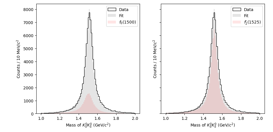
Now that we have the fitted free parameters, we can plot the result by calculating weights for the accepted Monte Carlo. This will be done using the NLL.project_weights method. Every amplitude in the model is either activated or deactivated. Deactivated amplitudes act like zeros in the model, so we can isolate certain amplitudes by passing them through the subset=... keyword argument for just a single calculation before reverting the NLL back to its prior state. If we need several projections at once, we can batch them with subsets=[...]. A None entry means “use the full currently active model”, so we can request the total and selected components in one call.

tot_weights, f0_weights, f2_weights = nll.project_weights(
    result.x,
    subsets=[
        None,
        ["[f_0(1500)]", "BW_0", "Z00+"],
        ["[f_2'(1525)]", "BW_2", "Z22+"],
    ],
)

fig, ax = plt.subplots(ncols=2, sharey=True)
# Plot the data on both axes
ax[0].hist(m_data, bins=100, range=(1.0, 2.0), color="k", histtype="step", label="Data")
ax[1].hist(m_data, bins=100, range=(1.0, 2.0), color="k", histtype="step", label="Data")

m_accmc = res_mass.value_on(accmc_ds)
# Plot the total fit on both axes
ax[0].hist(m_accmc, weights=tot_weights, bins=100, range=(1.0, 2.0), color="k", alpha=0.1, label="Fit")
ax[1].hist(m_accmc, weights=tot_weights, bins=100, range=(1.0, 2.0), color="k", alpha=0.1, label="Fit")

# Plot the f_0(1500) on the left
ax[0].hist(m_accmc, weights=f0_weights, bins=100, range=(1.0, 2.0), color="r", alpha=0.1, label="$f_0(1500)$")

# Plot the f_2'(1525) on the right
ax[1].hist(m_accmc, weights=f2_weights, bins=100, range=(1.0, 2.0), color="r", alpha=0.1, label="$f_2'(1525)$")

ax[0].legend()
ax[1].legend()
ax[0].set_ylim(0)
ax[1].set_ylim(0)
ax[0].set_xlabel("Mass of $K_S^0 K_S^0$ (GeV/$c^2$)")
ax[1].set_xlabel("Mass of $K_S^0 K_S^0$ (GeV/$c^2$)")
ax[0].set_ylabel(f"Counts / 10 MeV/$c^2$")
ax[1].set_ylabel(f"Counts / 10 MeV/$c^2$")
plt.tight_layout()
plt.show()

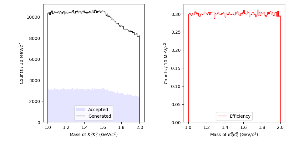
Notice that we have not yet used the generated Monte Carlo. We always assume that the generated Monte Carlo is distributed evenly in phase space, without any “physics” like resonances or spin. We can quickly plot the mass distributions for the Monte Carlo as well as the “efficiency” of the reconstruction per bin of mass:[2]

import numpy as np

m_genmc = res_mass.value_on(genmc_ds)
m_accmc_hist, mass_bins = np.histogram(m_accmc, bins=100, range=(1.0, 2.0))
m_genmc_hist, _ = np.histogram(m_genmc, bins=100, range=(1.0, 2.0))
m_efficiency = m_accmc_hist / m_genmc_hist

fig, ax = plt.subplots(ncols=2)
ax[0].stairs(m_accmc_hist, mass_bins, color="b", fill=True, alpha=0.1, label="Accepted")
ax[0].stairs(m_genmc_hist, mass_bins, color="k", label="Generated")
ax[1].stairs(m_efficiency, mass_bins, color="r", label="Efficiency")

ax[0].legend()
ax[1].legend()
ax[0].set_ylim(0)
ax[1].set_ylim(0)
ax[0].set_xlabel("Mass of $K_S^0 K_S^0$ (GeV/$c^2$)")
ax[1].set_xlabel("Mass of $K_S^0 K_S^0$ (GeV/$c^2$)")
ax[0].set_ylabel(f"Counts / 10 MeV/$c^2$")
ax[1].set_ylabel(f"Counts / 10 MeV/$c^2$")
plt.tight_layout()
plt.show()

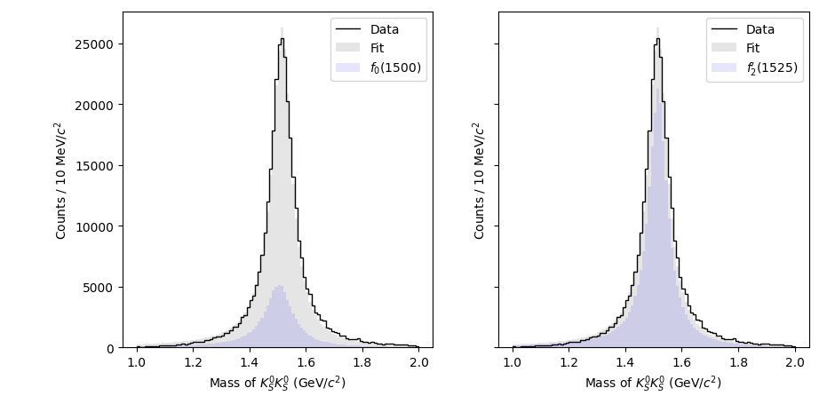
Finally, to project the fit result onto the generated Monte Carlo, we need to create an evaluator specifically for the generated Monte Carlo data. The reason this is done separately is that generated Monte Carlo datasets usually contain many events, so it’s sometimes more efficient to do the fit without loading this data at all, save the fit results, and plot the acceptance-corrected plots in a separate step, minimizing overall memory impact.

To create an Evaluator object, we just need to load up the model and dataset we want to use. All of these operations create efficient copies of the underlying expressions and data, so we don’t need to worry about duplicating resources or events.

gen_eval = model.load(genmc_ds)
tot_weights_acc, f0_weights_acc, f2_weights_acc = nll.project_weights(
    result.x,
    subsets=[
        None,
        ["[f_0(1500)]", "BW_0", "Z00+"],
        ["[f_2'(1525)]", "BW_2", "Z22+"],
    ],
    mc_evaluator=gen_eval,
)

# acceptance-correct the data distribution
m_data_hist, _ = np.histogram(m_data, bins=100, range=(1.0, 2.0))
m_data_acc_hist = m_data_hist / m_efficiency

fig, ax = plt.subplots(ncols=2, sharey=True)
# Plot the data on both axes
ax[0].stairs(m_data_acc_hist, mass_bins, color="k", label="Data")
ax[1].stairs(m_data_acc_hist, mass_bins, color="k", label="Data")

# Plot the total fit on both axes
ax[0].hist(m_genmc, weights=tot_weights_acc, bins=100, range=(1.0, 2.0), color="k", alpha=0.1, label="Fit")
ax[1].hist(m_genmc, weights=tot_weights_acc, bins=100, range=(1.0, 2.0), color="k", alpha=0.1, label="Fit")

# Plot the f_0(1500) on the left
ax[0].hist(m_genmc, weights=f0_weights_acc, bins=100, range=(1.0, 2.0), color="b", alpha=0.1, label="$f_0(1500)$")

# Plot the f_2'(1525) on the right
ax[1].hist(m_genmc, weights=f2_weights_acc, bins=100, range=(1.0, 2.0), color="b", alpha=0.1, label="$f_2'(1525)$")

ax[0].legend()
ax[1].legend()
ax[0].set_ylim(0)
ax[1].set_ylim(0)
ax[0].set_xlabel("Mass of $K_S^0 K_S^0$ (GeV/$c^2$)")
ax[1].set_xlabel("Mass of $K_S^0 K_S^0$ (GeV/$c^2$)")
ax[0].set_ylabel(f"Counts / 10 MeV/$c^2$")
ax[1].set_ylabel(f"Counts / 10 MeV/$c^2$")
plt.tight_layout()
plt.show()

Finally, we might want to save this fit result and refer back to it in the future. While Status objects directly support Python pickle serialization, there’s a shorthand method built in:

result.save_as("fit_result.pkl")
# This saves the minimization summary to a file called "fit_result.pkl"

saved_status = Status.load("fit_result.pkl")
# Now we've loaded that fit result again

This will create a rather small file, since the fit is not very complex, but saving multiple fits to a single file will become very useful when doing binned fits, which are the subject of the next tutorial.

Footnotes

[1]

In reality, there are many more resonances present in this channel, and the model we are about to construct technically doesn’t preserve unitarity, but this is just a simple example to demonstrate the mechanics of laddu.

[2]

In this toy example, the accepted Monte Carlo is just a random subset of the generated Monte Carlo, so the acceptance is approximately a constant 30% by construction. In reality, acceptance effects can be much more important than an overall scaling factor.

[Barlow]

Barlow, R. (1990). Extended maximum likelihood. Nuclear Instruments and Methods in Physics Research Section A: Accelerators, Spectrometers, Detectors and Associated Equipment, 297(3), 496–506. doi:10.1016/0168-9002(90)91334-8